Lecture 2: Introduction to R
RStudio · variables · vectors · data frames · live coding
2.1 Course objectives
- 2.1 Course objectives
- 2.2 Recap from Lecture 1
- 2.3 Introduction to R
- 2.4 Live Coding Session 1
- 2.M Conclusion of Lecture 2
Welcome to Finance Project — Asset Management
- This is a project course: there is no central exam to register for. Sign up on the course Moodle page by 15 April 2026 so you receive announcements and the data link.
- Submit the project by 30 June 2026 as a single zip — name pattern:
Asset2026_surname1_surname2_surname3. Email it to oliver.padmaperuma@uni-ulm.de, CC andre.guettler@uni-ulm.de and your team-mates.- Ask questions during or right after each session — that is the preferred channel.
- Admin / studies / exam-eligibility questions go to the registrar’s office (Studiensekretariat) at studiensekretariat@uni-ulm.de.
- Course-content questions outside class: email oliver.padmaperuma@uni-ulm.de, CC andre.guettler@uni-ulm.de.
- We also recommend the student advisory service.
Course Objective
Scope
We will:
- Build an end-to-end empirical pipeline in R: load, explore, model, back-test
- Cover the core ML toolbox for asset-management research: linear models, Ridge, Lasso, Elastic Net, cross-validation
- Apply it to a non-traditional asset class: prediction markets
- Develop your own indicator library and trading strategy in groups of three
We will NOT:
- Drift into deep-learning or reinforcement-learning methods
- Cover prediction markets in depth
- Provide a “ready-to-fork” backtest — the demo code is intentionally basic
Approach
Part I — Foundations
- L1: Motivation, organisation, backtesting fundamentals
- L2: Hands-on R intro — RStudio, live coding, etc.
- L3 + L4: Statistical learning — model accuracy, regularisation, resampling
Part II — Application
- L5: Prediction-markets primer + the Polymarket dataset + assignment briefing
- Project work in groups of three (≈ 7 weeks of self-organised work)
- Final session (1 July): 20-minute presentations per team
Course at a glance (1/2)
Foundations
Course outline · Backtesting fundamentals
- Course aim & organisation
- Backtesting overview & case study
- In-sample tests (Welch & Goyal 2008)
- Out-of-sample (walk-forward, R²_OS)
- Useful predictors & p-hacking
Introduction to R
RStudio · variables · vectors · data frames · live coding
- Why R for empirical asset-management research
- RStudio and the script editor
- Variables, vectors, matrices, data frames, lists
- Functions and loops
- Data import and export
Assessing model accuracy & Ridge regression
Statistical learning · MSE · bias-variance · linear model selection · Ridge
- Statistical learning: Y = f(X) + ε
- Quality of fit and the train/test MSE distinction
- Bias-variance trade-off and overfitting
- OLS limits: prediction accuracy & interpretability
- Ridge regression and the L2 penalty
Lasso, cross-validation & Elastic Net
Sparse regularisation · resampling for honest test error · choosing λ
- Lasso: L1 penalty and exact-zero coefficients
- Cross-validation: validation set, LOOCV, K-fold
- Choosing the optimal λ for Lasso
- OLS post-Lasso for cleaner coefficient inference
- Elastic Net — combining Ridge and Lasso
Prediction markets, the Polymarket Quant Bench & your project
From Welch-Goyal to event-resolved binary contracts
- Prediction markets — definition and Polymarket as the canonical venue
- How prices form: liquidity, resolution, mechanics
- The Polymarket Quant Bench dataset (HuggingFace): access and schema
- First look at the data in R
- Your project: indicator design, back-test, deliverables, R toolbox
Course at a glance (2/2)
Final presentations
Group presentations · Q&A · wrap-up
- Presentation order and time budget
- Q&A rules
- Closing thoughts and feedback
Assignments / Exams
Project (Code + Report) 50% of your grade
Rmd code + knitr-rendered PDF report. Build a library of indicators over the Polymarket Quant Bench dataset (curated OHLCV bars on HuggingFace, derived from Jon Becker’s polymarket-data dump), derive trade signals, back-test, and write a critical reflection.
Group of up to 3.
Submit by emailing oliver.padmaperuma@uni-ulm.de, CC andre.guettler@uni-ulm.de. Subject pattern: Finance Project — Asset Management_assignment-1-project-report_surname1_surname2_…
30 June 2026
Final Presentation 50% of your grade
20-minute group presentation in class on 1 July 2026; submit slides as PDF together with the project zip.
Group of up to 3.
Submit by emailing oliver.padmaperuma@uni-ulm.de, CC andre.guettler@uni-ulm.de. Subject pattern: Finance Project — Asset Management_assignment-2-final-presentation_surname1_surname2_…
1 July 2026
2.2 Recap from Lecture 1
- 2.1 Course objectives
- 2.2 Recap from Lecture 1
- 2.3 Introduction to R
- 2.4 Live Coding Session 1
- 2.M Conclusion of Lecture 2
What we covered last week
- Why we are here — develop indicator-based trading strategies for prediction markets in groups of three.
- Backtesting fundamentals — IS vs OOS tests, Welch and Goyal (2008) as the canonical empirical benchmark, \(R^2_{OS}\), walk-forward.
- Useful predictors checklist — significant IS and OOS, drift over multiple sub-samples, robustness in recent decades.
- P-hacking warning — multiple testing inflates false positives; the antidote is paper or real-money performance.
Notes
The Lecture 1 takeaways carry forward in three operational ways throughout the course:
- The four-criterion checklist for “useful predictor” — whatever indicator you build for the project, plan to evaluate it against IS significance, OOS R² > 0, drift across sub-samples, and continued OOS R² in the most recent sub-sample.
- Walk-forward backtesting — the project deliverable will require a walk-forward implementation, not a single full-sample fit. Lectures 3–4 introduce the modelling tools; Lecture 5 wires them into a walk-forward loop on the Polymarket data.
- P-hacking discipline — when you tune your indicator, log every variation you tried. The final report should be honest about what you tested, not just what worked. Multiple-testing corrections (Bonferroni, FDR, or White’s reality check) are the formal version of “be honest about your search”.
If the Lecture 1 material feels hazy, the Lecture 1 handout (handout.html) has the substantive prose under each slide — much more detailed than the in-class delivery.
Today’s roadmap
- Introduction to R — RStudio, packages, working directory, basic execution.
- Live coding session 1 — variables, vectors, matrices, data frames, lists, functions, loops, import / export.
The R basics that follow are shared with our sister course Research in Finance — the included partials are the canonical source. Edit them once and both courses stay in sync.
Notes
Two halves to today’s session:
- Part 1 — Introduction to R (slides under §2.3) — RStudio orientation, working directory, packages, the script-vs-console workflow, basic execution. If you have R experience already this is revision; if not, this is the conceptual setup before the live coding.
- Part 2 — Live coding (slides under §2.4) — variables, the four data types, vectors, matrices, data frames, lists, functions, loops, data import/export. Type along in your own RStudio session. Reading is not enough.
The shared R-basics partials are deliberately exhaustive — the goal is that you have a single reference handout (the rendered handout.html) that covers every R construct you’ll need for the rest of the course. The next lectures (regression, ridge, lasso, cross-validation) all assume R fluency at this level; spending the time today is a high-leverage investment for the rest of the term.
2.3 Introduction to R
- 2.1 Course objectives
- 2.2 Recap from Lecture 1
- 2.3 Introduction to R
- 2.4 Live Coding Session 1
- 2.M Conclusion of Lecture 2
Survey — let’s get to know you
Open the Mentimeter link shared in class.
Notes
A short Mentimeter survey at the start of the session — degree program, prior coding language, prior exposure to R or Python — calibrates how fast we can move. R syntax is forgiving once you have written code in any language; if this is your first programming experience, the friction is usually the workflow (saving scripts, the working-directory concept, package management) rather than the statistics. Run every code chunk in your own RStudio session as we go through the deck — passive reading is much less effective than typing the lines and watching the output appear.
Why learn R?
- It’s free and open-source.
- A powerful tool for data analysis and graphics.
- R code is great for reproducibility and shareability — submit your script and anyone can re-run your results.
- A large, active community continuously extends R via packages.
- Widely used in academia and industry — especially in finance, economics, and data science.
Notes
R is the lingua franca of empirical statistics in academia and dominates academic finance research alongside Python and Stata. The “free and open-source” point is more consequential than it sounds: any result you produce in R can be re-run by an editor, reviewer, or replicator anywhere in the world with no licence cost — that is one of the foundations of reproducible research (Scheuch, Voigt, and Weiss 2023). The package ecosystem is the second killer feature: you do not write portfolio construction or panel regression from scratch — you load tidyquant, plm, fixest, tidyverse and stand on others’ work, freeing you to focus on the empirical question.
For empirical finance specifically, Tidy Finance with R (Scheuch, Voigt, and Weiss 2023) gives a free, end-to-end pipeline (downloading prices from WRDS, building factor portfolios, estimating Fama–MacBeth regressions) that mirrors the workflow you will use in the assignment. R for Data Science (Wickham and Çetinkaya-Rundel 2023) is the canonical introduction to the broader tidyverse stack and is also free online.
What are R and RStudio?
- R is a programming language for statistical computing, data analytics, and scientific research. It is one of the most widely used languages by statisticians and researchers to manage, manipulate, analyze, and visualize data.
- RStudio is an integrated development environment (IDE) for R that makes interaction with R easier — code completion, debugging, project management, plot viewing.
- In 2022 RStudio was rebranded Posit to signal its move toward language-agnostic tooling.
In order to use RStudio, you need to have R installed. RStudio is just the interface. R does the actual computing.
Notes
R is the language and the runtime; RStudio is just an editor wrapping that runtime. You can run R from a plain terminal with no IDE (typing R at a shell prompt drops you into a REPL), but the RStudio pane layout — script editor + console + environment + viewer — is the standard interactive workflow and what every R tutorial assumes. Think of the relationship as Word vs. the underlying typesetting engine: the editor makes life nicer but the engine does the work.
The 2022 rebrand from “RStudio” (the company) to Posit reflects the company’s pivot to multi-language tooling — Quarto, the system that produces these slides, can author documents in R, Python, Julia, and Observable JS through the same interface. The IDE itself is still called “RStudio Desktop” — you will see “Posit” on the download page and in newer package release notes, but it’s the same product students have been using for a decade.
Installing R and RStudio
- Go to https://cran.r-project.org/ and click Download R for Windows / macOS.
- Click base subdirectory.
- Click Download R-x.x.x for Windows and run the
.exe. Accept defaults. - Go to https://posit.co/download/rstudio-desktop and click Download RStudio.
- Run the RStudio installer.
Notes
Two installations, in this order: R first, then RStudio. RStudio auto-detects your R installation on launch but does not ship a copy of R itself, which is why the order matters. On Windows the default install path is C:\Program Files\R\R-x.x.x\; on macOS it’s /Library/Frameworks/R.framework/. If you already have an older R version, leave it installed alongside the new one — Tools → Global Options → General → R version in RStudio lets you pick which R the editor uses per project, useful when you need to reproduce something written against an older R.
University-managed or corporate laptops occasionally block CRAN downloads with proxy or certificate errors. If install.packages() fails with unable to verify the first certificate or similar, try chooseCRANmirror() and pick a different mirror, or pin one in your .Rprofile with options(repos = c(CRAN = "https://cloud.r-project.org")). The Posit-hosted “cloud” mirror is the most reliable default.
RStudio interface
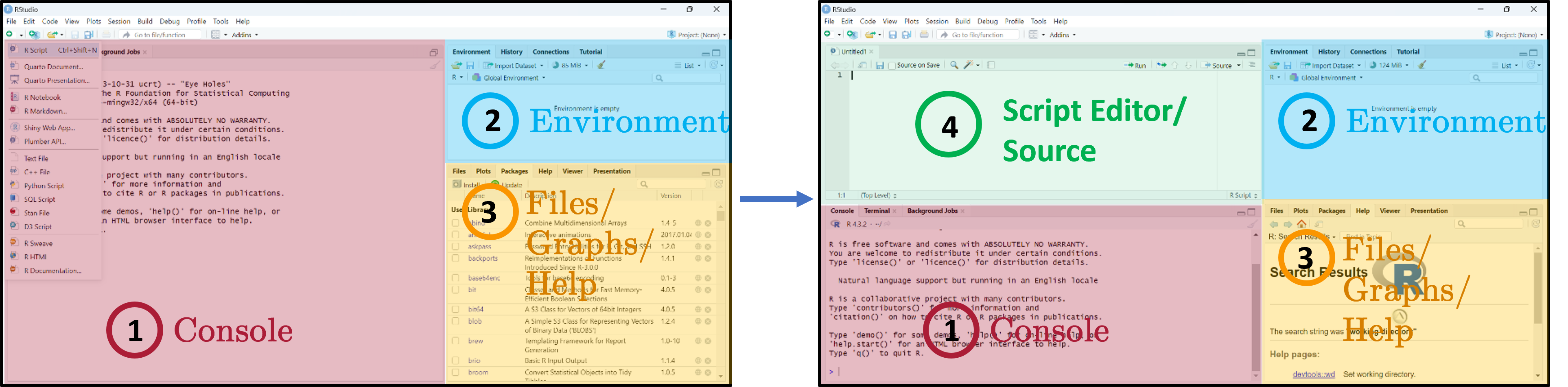
Three main panes when you open RStudio:
- Console — where R code is executed.
- Global Environment / History — your in-memory objects.
- Files / Plots / Packages / Help / Viewer — the swiss-army-knife pane.
- Script Editor — where you write and save your R scripts.
Notes
The four-pane layout is the workflow you will use every session, so it pays to internalise it now:
- Script Editor (top-left) — where your
.Rfiles live and persist on disk. This is the source of truth for any analysis you intend to keep or share. - Console (bottom-left) — the live R process. Anything you run from the script editor is sent here for execution; you can also type ad-hoc commands directly. Console history evaporates when you quit RStudio, so do not rely on it for anything you want to repeat.
- Environment / History (top-right) — every object currently in memory (data frames, vectors, fitted models). Click an object’s name to inspect it without typing a
View()call. - Files / Plots / Packages / Help / Viewer (bottom-right) — Plots holds the most recent figure (use the broom icon to clear), Help renders
?function-namelookups, Packages lets you install/load with checkboxes (handy but bypasses your script — preferlibrary()calls inside your script for reproducibility).
Drag the divider bars to resize panes; View → Panes → Pane Layout lets you rearrange them.
Writing code in RStudio
- Load and save
.Rscripts. - Keeps a record of your analysis — show others how it was run, repeat later.
- Edit code without accidentally running it.
- Where R code is executed.
- You can also run code interactively here, but it is NOT saved on disk.
- See output and errors directly.
Write and run code through the Script Editor. Use the Console only for quick exploration.
Notes
This split is one of the most important workflow habits to develop early: the script is your analysis, the console is a scratchpad. A common student mistake is typing data <- read.csv(...) in the console, getting it to work, and never moving the line into a script — the next day, after a restart, the data frame is gone and there is no record of how it was loaded.
Every command that produces a result you want to be able to reproduce belongs in a .R script, run by sending it to the console with Ctrl/Cmd + Enter. The console is for ?function-name lookups, quickly checking head(data), doing 2 + 2-style arithmetic — anything ephemeral. When you submit your assignment, the marker should be able to take just your .R script and the input data, run it from a fresh R session, and reproduce all of your results without touching the console.
Setting the working directory
# Option 1: menu
# Session → Set Working Directory → Choose Directory…

# Option 2: code
setwd("C:/Users/<you>/Documents/research-in-finance")

# Verify
getwd()- The working directory (
wd) is where R looks for and saves files. - Two ways to set it: via the menu, or in code with
setwd(). - Always verify with
getwd()to avoid confusion about where your files are being read from or written to. - Tip: set the working directory at the start of your script so it’s clear where files are coming from and going to. Avoid hardcoding paths if you plan to share your code with others or run it on different machines.
Notes
The working directory is the folder R uses as the implicit base for any relative path you give it: read.csv("prices.csv") reads prices.csv from the current working directory; write.csv(out, "results.csv") writes there too. Most “file not found” errors in introductory R are working-directory problems — R is looking somewhere different from where you think.
setwd() with a hard-coded absolute path is the quick fix shown on this slide, but it has a serious drawback: the path is specific to your machine, so a co-author or marker who runs your script will hit a missing-folder error immediately. Two cleaner alternatives that you should adopt as soon as you are comfortable:
- RStudio Projects (
File → New Project…) — creates a.Rprojfile in a folder; opening it sets the working directory to that folder automatically. Sharing the folder shares the project, and the script’s relative paths just work on any machine. - The
here::here()function —read.csv(here("data", "prices.csv"))resolves relative to the project root regardless of where the script is being executed from. Particularly useful in larger projects withdata/,code/,output/subfolders.
Avoid hard-coding C:\Users\you\… paths in any script you intend to share. The very first line of every script should make the data location explicit and portable.
Getting started — running code
The blinking cursor in the Script Editor prompts you to write. The Console shows > when R is ready.
Four ways to run code:
- Ctrl/Cmd + Enter — run current line / selection.
- Click Run.
- Ctrl + Shift + Enter — run all lines in the editor.
- Highlight lines and click Run.
Type 1 + 2*8 and log(10). Result appears in the Console with a leading [1] (the index of the first element on that line).
Notes
The > prompt means R is idle and ready for input. A + prompt instead means R thinks the previous statement is incomplete and is waiting for you to finish it — the most common cause is an unclosed parenthesis or quote. Press Esc to abandon the half-finished command and get the > prompt back.
The bracketed [1] at the start of console output is just the index of the first element printed on that line — when you print a long vector that wraps across several console lines, each new line starts with the index of its first element ([14], [27], …). For a single-value result like log(10) it always shows [1] because there is only one element. It is not a footnote or warning marker, just a navigation aid for long vectors.
Ctrl/Cmd + Enter is the workflow keystroke you will use thousands of times — it sends the line under the cursor (or the highlighted region) to the console, executes it, and advances to the next line. Practising this from session one builds the reflex.
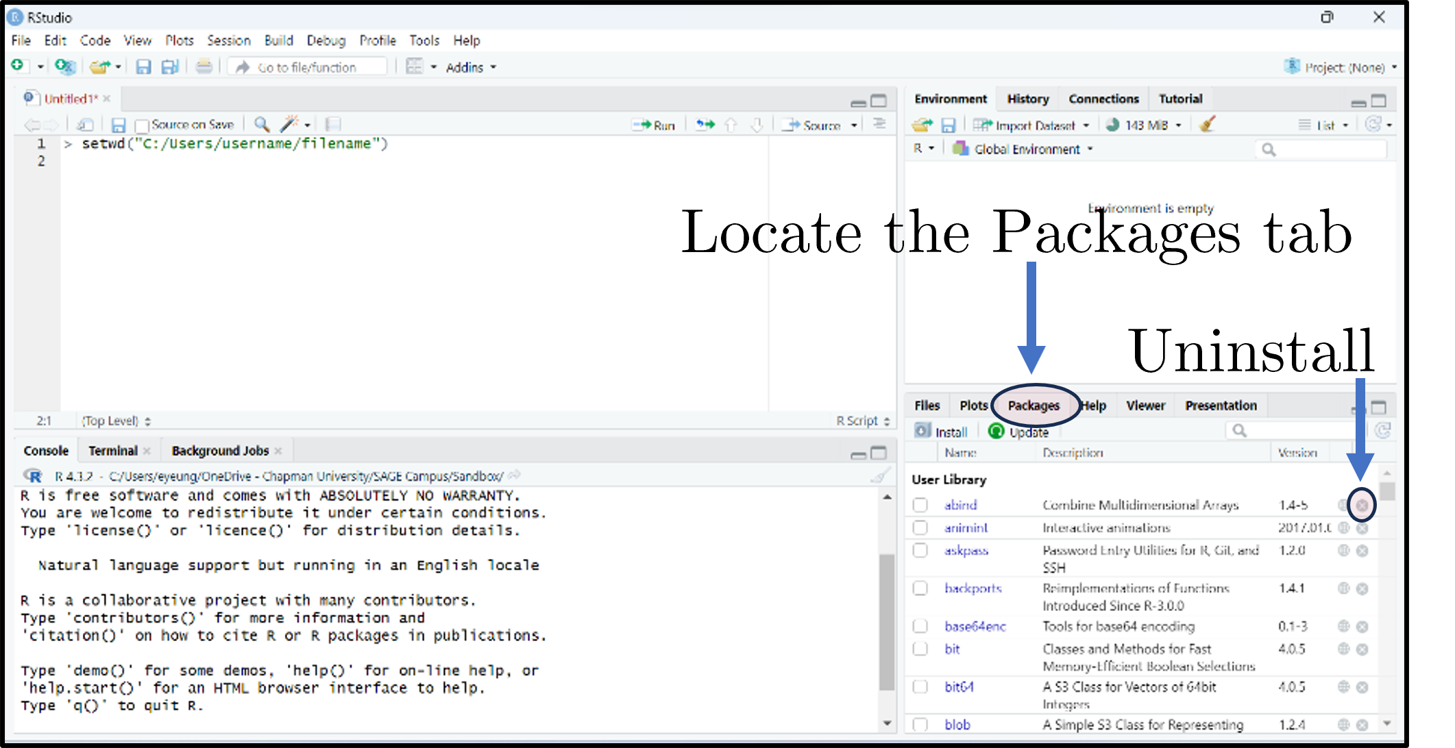
What are packages?
- Packages expand what you can do beyond base R.
- A collection of functions, data sets, and other R objects under one name.
- Install from repositories: CRAN, GitHub, etc.
- The Packages tab lists installed packages; click Update to upgrade; the small × uninstalls.
Notes
“Base R” — what you get out of the install — covers core data structures, basic plots, and standard statistical models (linear regression, t-tests, ANOVA). Almost any modern empirical workflow goes beyond that, and packages are how the community ships extensions: a package is a folder of functions, datasets, documentation, and tests bundled with metadata about its dependencies.
The two repositories you will encounter most:
- CRAN — the Comprehensive R Archive Network, the official curated repository. CRAN runs automated checks before accepting a package, which gives a baseline quality guarantee but means CRAN versions can lag development by weeks or months. Most production work uses CRAN packages.
- GitHub — many packages are developed on GitHub and you can install pre-release versions with
remotes::install_github("owner/repo"). Useful for bleeding-edge features or for packages that have not yet been published to CRAN.
A minimum-viable workflow for empirical finance pulls in the tidyverse (data manipulation + plotting), tidyquant (price data), and a regression-tools package such as fixest or plm. R for Data Science (Wickham and Çetinkaya-Rundel 2023) walks through the tidyverse stack in detail.
Installing and loading packages
install.packages("tidyverse")
install.packages("tidyquant")
install.packages("Quandl")
Or click Install in the Packages tab.
library(tidyverse)
library(tidyquant)
library(Quandl)
Or tick the package’s checkbox in the Packages tab.
Install and load the tidyverse, tidyquant, and Quandl packages.
Notes
The two-step distinction trips up beginners constantly: install.packages() downloads and installs the package once (it lives in your R library on disk thereafter); library() loads it into the current R session (makes its functions available to call). You install once per machine; you load once per script.
Convention is to put all library() calls at the top of the script — that way a reader can see at a glance which packages your code depends on, and an attempt to run the script in a fresh session fails fast with a clear “package X not installed” error rather than a confusing “function not found” much later. Do not put install.packages() calls in your script — they would re-download the package every time anyone runs it. The reader is responsible for installing the dependencies your script declares.
If library(tidyverse) complains “there is no package called ‘tidyverse’”, you have not run install.packages("tidyverse") yet on this machine. If install.packages() itself fails, see the proxy / mirror notes from the installation slide above.
2.4 Live Coding Session 1
- 2.1 Course objectives
- 2.2 Recap from Lecture 1
- 2.3 Introduction to R
- 2.4 Live Coding Session 1
- 2.M Conclusion of Lecture 2
Creating objects / variables
# Practice
x <- 5
x + x   # → [1] 10
y <- x * 2
y # → [1] 20- The “<-” operator assigns the value on the right to the name on the left.
- Avoid long object names, be descriptive
- Don’t reuse names of existing R functions
- No blank spaces - use
_or. - R is case-sensitive (
xandXare different) - Use
=for function arguments, but “<-” for assignment to avoid confusion - Don’t use
=for assignment in scripts, as it can lead to bugs and readability issues
Notes
The <- arrow is R’s traditional assignment operator and is the convention almost every R style guide recommends; = also assigns at the top level but its primary purpose is naming arguments inside function calls (mean(x, na.rm = TRUE)). Mixing the two is legal but reads as sloppy in code review and makes it harder to spot bugs — settle on <- for assignment from day one. RStudio’s Alt + - keyboard shortcut inserts <- with surrounding spaces.
Naming: case-sensitive, so Returns and returns are different objects. The accepted style is snake_case (monthly_returns) or, less commonly, camelCase (monthlyReturns); never spaces (monthly returns is illegal) and avoid dots (monthly.returns) because dots have special meaning in S3 method dispatch (print.data.frame). Avoid shadowing built-ins — naming a vector c or data works but breaks code that calls the homonymous function c() or data(). When in doubt, run ?name first; if R has a help page for it, pick a different name.
Four data types in R
- Numeric — numbers that may contain decimals.
- Integer — special case, no decimals (suffix
L).
- Integer — special case, no decimals (suffix
- Character — text (strings); wrap in
" ". - Factor — special character used for categorical data (e.g., male/female, months).
- Logical — Boolean (
TRUE/FALSE).
class(objectname)returns the higher-level label R uses to decide which functions and behaviors apply ("data.frame","factor","matrix","numeric").
Notes
The four atomic types are the building blocks of every more complex structure (vectors, matrices, data frames). For empirical finance the type that surprises new R users most is the factor — it looks like character text but R stores it as integers under the hood with a separate “levels” attribute, and many statistical functions (lm, glm, aov) treat factors specially when they appear as predictors (creating dummy variables automatically). Read a CSV containing strings via read.csv(...) and depending on your R version columns may be silently coerced to factor or kept as character; check with str(df) early.
Numeric vs. integer rarely matters in practice — R promotes integers to numeric in any arithmetic involving non-integer values — but it occasionally bites when interfacing with C code or databases. The L suffix (10L) is the explicit integer literal. Logical is the type R returns from comparisons (x > 5) and the input boolean filters expect (subset(df, df$age > 18)).
class() answers “what is this for the dispatch system” and is what most code cares about; typeof() answers “what is the underlying storage type” and is more useful when debugging weird behaviour.
Variables and basic operations
myNumber  <- 3      # numeric (default)
myInteger <- 10L    # integer ('L' suffix)
myText    <- "Some sentence..."   # character
myFactor  <- factor(c("red", "blue", "red", "green")) # factor
levels(myFactor)    # "blue" "green" "red"
myLogical <- TRUE # logical- Assign and compute financial metrics — returns, prices, ratios — quickly during empirical work
- Use factors to manage categorical variables like sectors, credit ratings, or time periods
- Logical variables are useful for filtering data frames (e.g.,
subset(myData, myData$sector == "Tech"))
Notes
A typical finance use of factors: rating bins (AAA, AA, A, …). Storing them as a factor with explicitly ordered levels lets you compute conditional statistics by rating in one call (tapply(spread, rating, mean)), produce neatly ordered plots, and keep the order stable when you subset (subsetting a character vector loses unobserved categories; subsetting a factor preserves them in levels() until you droplevels()).
Logical vectors are the basis of subsetting in base R: myData[myData$sector == "Tech", ] reads as “from myData, the rows where sector equals "Tech", all columns”. Each element of myData$sector == "Tech" is TRUE/FALSE, and the row index […, ] keeps rows where that boolean is TRUE. The same logic is the engine behind subset(), dplyr::filter(), and the [] operator throughout R — once it clicks, most data-cleaning operations become one-liners.
Five basic data structures
- Individual values — single scalars.
- Vectors — ordered collections of elements (one type only).
- Matrices — 2D arrays; rows × columns; one type only.
- Data frames — like spreadsheets; columns can have different types.
- Lists — flexible containers that can hold vectors, matrices, data frames, even other lists.
Notes
Pick the structure that fits the data: numeric vectors for time series of returns, matrices for correlation/covariance matrices, data frames for everything that comes out of a CSV (mixed-type columns), lists for collections of unlike objects (e.g., a fitted regression model — which is itself a list of coefficients, residuals, fitted values, etc.).
There is no atomic “scalar” type in R — what looks like a single value is just a length-1 vector. length(5) returns 1, and 5[1] works. This unifies a lot of R’s behaviour: a function that takes a vector accepts a scalar without any special case. The trade-off is occasionally surprising error messages when you forgot you were passing a vector.
The data frame is by far the structure you will use most in empirical finance. The modern tibble (from the tidyverse) is a slightly more pleasant variant: identical for most purposes, but with cleaner printing and stricter subsetting rules — see (Wickham and Çetinkaya-Rundel 2023) for the full comparison.
Vectors
# Create
myVector <- c(3, 4, -1.1, pi)

# Inspect / aggregate
myVector[3]        # third element: -1.1
length(myVector)   # 4
sum(myVector)      # ~9.04
mean(myVector)     # ~2.26
var(myVector)      # ~5.21
sort(myVector)     # ascending: -1.1, 3.0, 3.14, 4.0
quantile(myVector, c(0.1, 0.25, 0.95))

# Vectorized arithmetic — no loops needed
myVector + 2
myVector * myVector

# Coercion: mixed types collapse to character
mixed <- c(1, "two", TRUE)   # "1" "two" "TRUE"

# Named vectors
namedVec <- c(apple = 5, banana = 3)
namedVec["banana"] # 3- Basic syntax:
c()combines values into a vector; indexing with[]retrieves elements - Vectors are the building blocks of more complex structures. They allow you to store and manipulate sequences of numbers, text, or logical values efficiently
- Vectorized operations enable you to perform calculations on entire vectors without writing explicit loops, which is faster and more concise
- Named vectors can improve readability and allow for easier access to specific elements by name rather than index
Notes
Vectorisation is the single most important R idiom to internalise: arithmetic and most functions apply element-wise to whole vectors at once, with no for loop required. myVector * 2 doubles every element in a single C-level operation; the equivalent loop in R-level code would be 100x slower on a vector of any meaningful length. Almost every finance function in base R and the tidyverse is vectorised — pmin(), cummax(), lag(), diff(), cumprod() for compounding returns, quantile() for risk measures.
R’s coercion rule for mixing types in c() is “promote to the most general type that can hold all values” — so any character forces the whole vector to character, any numeric (with no character) forces logicals to numeric. This is silent, which means c(1, "two", TRUE) yields c("1", "two", "TRUE") without warning. Always check class(myVector) after assembling a vector if you are unsure of types.
Indexing in R uses 1-based subscripts: myVector[1] is the first element. Negative indices remove (myVector[-1] is everything except the first); logical vectors filter (myVector[myVector > 0]); names index by name (namedVec["banana"]). These four indexing modes (positive integer, negative integer, logical, name) are the same across every R container.
Matrices
myMatrix <- matrix(c(2, 1, 0, -9, 5, 0), nrow = 2, byrow = TRUE)
dim(myMatrix)              # [1] 2 3
myMatrix[1, 1] <- 2.1415   # modify cell
myMatrix[, 2]              # second column

# Linear algebra
anotherMatrix <- matrix(c(5, -1, 7, 0, 2, -1), nrow = 2, byrow = TRUE)
transposedMatrix <- t(anotherMatrix)
matrixProduct    <- myMatrix %*% transposedMatrix     # 2x2 product
matrixInverse    <- solve(matrixProduct)              # inverse

# Aggregations
rowSums(myMatrix)
colMeans(myMatrix)

# Bind: combine rows / cols
cbind(myMatrix, c(6, 7))- Basic syntax:
matrix()creates a matrix from a vector of values; specifynrowandncolto set dimensions;byrow = TRUEfills by rows instead of columns - Matrices are 2D structures that can only hold one type of data (e.g., all numeric)
- They are essential for linear algebra operations, which are common in finance1
- Functions like
rowSums(),colMeans(), andcbind()allow you to perform common matrix manipulations without writing loops
Notes
Use a matrix instead of a data frame when (a) every cell is the same type (typically numeric) and (b) you need linear-algebra operations. The classic finance examples: a covariance matrix (rows and columns indexed by asset, cells holding \(\\sigma_{ij}\)), a portfolio-weights vector multiplied by an asset-returns matrix (weights %*% returns_matrix), or solving a system \(\\Sigma w = \\mu\) for mean-variance weights via solve(Sigma, mu).
The key linear-algebra operators: t() transposes; %*% is matrix multiplication (do not use *, which is element-wise); solve(A) returns \(A^{-1}\), and the more numerically stable solve(A, b) returns \(A^{-1}b\) in one step (preferred for solving systems). For large matrices in production code, look at the Matrix package which exploits sparsity.
byrow = TRUE is worth flagging: by default matrix() fills column-by-column (R’s column-major storage), which is unintuitive when you write the values out as a literal that “looks like” a row-by-row matrix in source. Always pass byrow = TRUE if your literal reads naturally row-by-row.
Data frames
student_name <- c("Student A", "Student B", "Student C")
grade        <- c(1.7, 2.3, 5.0)
students     <- data.frame(student_name, grade)

students$grade                    # column access
colnames(students)[2] <- "exam2021"
students[2:3, ]                   # rows 2-3

# Add columns
students$degree    <- c("Bachelor", "Master", "Bachelor")
students$pass_fail <- c("Pass", "Pass", "Fail")
table(students$degree, students$pass_fail)

# Summary
summary(students)

# Subset by condition
subset(students, exam2021 > 2)

# Add row
newStudent <- data.frame(student_name = "Student D", exam2021 = 3.5,
                         degree = "PhD", pass_fail = "Pass")
students <- rbind(students, newStudent)

# Merge with another frame
ages   <- data.frame(student_name = c("Student A", "Student B", "Student C"),
                     age = c(20, 22, 21))
merged <- merge(students, ages, by = "student_name")- Basic syntax:
data.frame()creates a data frame from vectors; columns can have different types; access with$or[] - Data frames are the most common structure for tabular data in R. They can hold different types of data in different columns (e.g., numeric grades, character names, factors for degree)
- Adding new columns is straightforward, and you can easily summarize or subset the data
- Merging data frames is common when you have related datasets2 that share a key
Notes
The data frame is the workhorse of empirical finance — every CSV / Stata file / SQL query result you load arrives as one. Conceptually it is a list of equal-length columns, each of which can be a different type. That mixed-type capability is what distinguishes it from a matrix and is what makes it the right structure for typical financial datasets (string ticker, integer date, numeric price, factor sector all in one row).
Three operations you will use constantly:
merge(x, y, by = "key")— the SQLINNER JOIN. Passall.x = TRUEfor a left outer join,all = TRUEfor a full outer join. The tidyverse equivalents (dplyr::left_join,inner_join,full_join) read more cleanly when you chain multiple joins.subset(df, condition)— keep rows matching a logical condition. The tidyverse version isdplyr::filter(). Both internally dodf[condition, ].summary(df)— quick per-column descriptive statistics. Useful first-pass look at a new dataset; for serious EDA reach forskimr::skim()orHmisc::describe()instead.
The example uses base R; the tidyverse introduces an alternative grammar (mutate, filter, select, summarise chained with %>% or |>) that we will rely on heavily in later lectures and that Tidy Finance with R (Scheuch, Voigt, and Weiss 2023) uses throughout.
Lists
scoresList <- list(
  scores = c(95, 85, 92),
  names  = c("Alice", "Bob", "Carol"),
  passed = c(TRUE, TRUE, FALSE)
)

str(scoresList)

scoresList$scores[3] <- 90  # update Carol's score
scoresList$comments  <- "All passed"  # add element

# Nested list
nestedList <- list(course = "Math 101", details = scoresList)
nestedList$details$names[1]  # "Alice"

# Convert to data frame (elements need equal length)
scoresDF <- as.data.frame(scoresList)- Basic syntax:
list()creates a list; access with$or[]; lists can contain any type of object, including other lists - Lists are flexible containers that can hold a variety of objects, making them useful for storing complex data structures or results from functions that return multiple outputs
- They are particularly useful when you want to return multiple related objects from a function without having to combine them into a single data frame or matrix
Notes
Lists are the escape hatch for “I need to bundle several unrelated objects together”. The most common case in practice is a fitted model: when you call lm(y ~ x, data = df), R returns a list containing coefficients, residuals, fitted values, the model frame, the call, etc. — class(fit) reports "lm" but typeof(fit) is "list". That is why fit$coefficients works and why most extractor functions (coef(), residuals(), predict()) are essentially typed accessors over the underlying list.
[[ ]] versus [ ] on a list is a notorious gotcha: mylist[[1]] extracts the contents of the first element (whatever its type was); mylist[1] returns a list of length 1 containing that element. The first is what you usually want for further computation; the second is for sub-setting. $name is shorthand for [["name"]].
str(list_object) is the indispensable debugging tool — it prints the full nested structure with types and a few values per leaf. Use it whenever a function returns something complicated and you are not sure what is inside.
Functions
# Define
bmiCalc <- function(height, weight) {
  bmi <- weight / (height ^ 2)
  return(round(bmi, 1))
}

# Call
myBmi <- bmiCalc(1.75, 70)   # 22.9

# Default arguments
bmiCalcDefault <- function(height, weight = 70) {
  round(weight / (height ^ 2), 1)
}
bmiCalcDefault(1.75)         # 22.9

# Multiple returns via list
bmiAdvanced <- function(height, weight) {
  bmi <- weight / (height ^ 2)
  category <- ifelse(bmi < 18.5, "Underweight",
                     ifelse(bmi < 25, "Normal", "Overweight"))
  list(bmi = round(bmi, 1), category = category)
}
result <- bmiAdvanced(1.75, 70)
result$bmi        # 22.9
result$category # "Normal"- Basic syntax:
function(arg1, arg2) { ... }defines a function; usereturn()to specify output; functions can have default arguments and return multiple values via lists - Functions allow you to encapsulate reusable code, making your scripts cleaner and more modular
- Functions are essential for performing repeated calculations, especially when you need to apply the same logic to different inputs
Notes
Two language details worth knowing from the start:
- Implicit return. R’s
return()is optional — a function returns the value of its last evaluated expression. Many R programmers omitreturn()for a one-liner (bmiCalc <- function(h, w) round(w / h^2, 1)) and use it only when control flow demands an early exit. Both styles are correct; pick one and stay consistent within a script. - Lexical scope. A function can read variables from the environment in which it was defined — useful for building up parameterised helpers, but a footgun if you accidentally rely on a global. As a rule, every input the function needs should be an explicit argument. If you find yourself referencing a free variable inside a function body, refactor it into an argument.
Returning multiple values via a list (the bmiAdvanced pattern) is the standard R idiom — there is no tuple type. Callers unpack with result$bmi, result$category, or destructure via with(). For functions that compute a “main” result plus diagnostics, the convention is to return the main value and attach diagnostics as attr(result, "diagnostics") <- list(...); many base-R functions (scale, lm) follow this pattern.
Loops
nums <- c(1, 2, 3, 4, 5)

# For-loop: sum even numbers
evenSum <- 0
for (i in nums) {
  if (i %% 2 == 0) evenSum <- evenSum + i
}
evenSum    # 6

# While-loop
j <- 1
while (j <= 3) {
  print(j)
  j <- j + 1
}

# Nested for-loop
for (a in 1:2) {
  for (b in 3:4) {
    print(a * b)   # 3, 4, 6, 8
  }
}- Basic syntax:
for (var in sequence) { ... }iterates over elements;while (condition) { ... }continues until condition is false - Loops are useful for certain tasks, but in R, they can be inefficient for data manipulation. Whenever possible, use vectorized operations or apply functions instead of loops for better performance
- In practice, you’ll often use functions from packages like
dplyrthat abstract away the need for explicit loops when working with data frames
Notes
The conventional R wisdom — “loops are slow, vectorise instead” — is half true. The slow part is not the for keyword itself; it is growing a result inside the loop without pre-allocating, which forces R to copy the entire result vector at every iteration. Compare:
# Slow — vector grows each iteration, copying every time
out <- c()
for (i in 1:1e5) out <- c(out, i^2)

# Fast — pre-allocate, then assign in place
out <- numeric(1e5)
for (i in seq_along(out)) out[i] <- i^2

# Fastest — vectorised: one call, no R-level loop
out <- (1:1e5)^2
The first form is O(\(n^2\)); the second is O(\(n\)); the third is O(\(n\)) but executed in C. Always prefer vectorised code when it exists; pre-allocate when you do need a loop.
The functional alternatives — sapply, vapply, lapply, mapply in base R; purrr::map(), map_dbl(), map2() in the tidyverse — are not faster than a pre-allocated for-loop, but they read more cleanly because intent (apply this function to each element) is explicit. R for Data Science (Wickham and Çetinkaya-Rundel 2023) has a chapter on purrr worth reading once you are comfortable with vectors.
Data import & export — file types
You will rarely build matrices/data frames by hand. Common ways to read data:
- Text —
.TXT(readLines()) - Tabular —
.CSV,.TSV(read.table(),readr::read_csv()) - Excel —
.XLSX(xlsx,readxl) - Google sheets —
googlesheets4 - Statistics programs — SPSS, SAS (
haven) - Databases — MySQL (
RMySQL)
Notes
The format-by-format menu reflects the ecosystem: in academic finance you will spend most of your time on CSVs (the WRDS export format), occasional Excel files (analyst spreadsheets, central-bank releases), and increasingly Parquet (the columnar binary format used by the Polymarket dataset later in the term — read with arrow::read_parquet()).
Two practical choices worth making early:
- Prefer
readr::read_csv()over baseread.csv()— it is faster on large files, doesn’t auto-coerce strings to factors, reports column types in a clear summary, and handles dates and large integers more sensibly. The tidyverse install pulls it in. - Avoid building a data frame “by hand” with literal vectors. It is tempting for tiny illustrative examples, but in real work you load from disk. If you ever find yourself typing a CSV-like literal into your script, that data should be in a CSV next to the script instead — the script then becomes generic and re-runnable on updated input.
Data import & export — examples
# CSV
objectname <- read.csv("your_file.csv", header = TRUE)

# Tab-delimited
objectname <- read.table("your_file.txt", sep = "\t", header = TRUE)

# Excel
library(readxl)
objectname <- read_excel("your_file.xlsx")

# RDS (R single-object binary)
objectname <- readRDS("your_file.rds")
# CSV
write.csv(objectname, file = "output_file.csv", row.names = FALSE)
# Tab-delimited
write.table(objectname, file = "output_file.txt",
sep = "\t", row.names = FALSE, col.names = TRUE)
# Excel
library(writexl)
write_xlsx(objectname, "output_file.xlsx")
# RDS
saveRDS(objectname, file = "output_file.rds")The argument
sep =may not be necessary — R recognises,in.csvand whitespace in.txt. But sometimes R won’t read correctly unless you specify it
Notes
Two common gotchas on this slide:
row.names = FALSEwhen writing CSVs — without it,write.csv()adds an unwanted leading column with the row numbers1, 2, 3, …that the next reader of the file has to clean up. Always set it. (readr::write_csv()does the right thing by default.).RDSis for intermediate / cached results, not for sharing data with non-R users. It is R-specific: you cannot open an.rdsin Excel or Python. Use it when you have an expensive computation (e.g. a fitted model on millions of rows) that you want to cache between R sessions; use CSV / Excel / Parquet for anything that crosses tool boundaries.
The Excel readers (readxl::read_excel, writexl::write_xlsx) are pure-R/C++ and have no Java dependency — they replace the older xlsx package which required rJava and was a frequent install nightmare. Prefer the modern packages.
Saving your script
- Save every step in an
.Rscript. Comment lines start with#and are ignored at run time. - File → Save, or click the disk icon, or Ctrl/Cmd + S.
- Unsaved scripts (or unsaved edits) show red text and an asterisk in the tab name.
Notes
The script is your scientific record — at the end of a project the script (plus the input data) should be sufficient for any colleague to reproduce your every result. Two habits make this real:
- Save often (
Ctrl/Cmd + S). RStudio does not auto-save by default; the asterisk on a tab title means there are unsaved changes that would be lost in a crash. - Comment liberally. Every code block should have at least a one-line
# … explains whycomment. Comments document intent, which the code itself does not — six months later, “why did I winsorise at 1%?” is a question only the comment can answer.
Once you start working on something more than a one-off script, graduate to R Projects (File → New Project) and version control with Git. Both are covered later in the course, but adopt the project pattern early — it solves the working-directory problem (the previous slide) and makes it natural to ship a single self-contained folder when you submit the assignment.
Closing an R session
Three ways to close RStudio:
- File → Quit Session
- The red ✕ in the top-right corner.
- Run
q()in the Console.
Unless (a) you ran something very expensive, or (b) you’re nearly done with the project. Starting clean each session avoids hidden state from previous runs.
Notes
The “save workspace image?” prompt is one of R’s most consequential defaults. If you say Yes, RStudio writes every object in your current session to a hidden .RData file and reloads it on next startup — meaning your next session starts with whatever variables happened to be lying around when you quit, not a clean state.
This breaks reproducibility silently: code that “worked” yesterday because some variable was in memory will fail today on a colleague’s machine that does not have that variable. The professional habit is to always say No to this prompt, and to disable the auto-load globally in Tools → Global Options → General: untick “Restore .RData into workspace at startup” and set “Save workspace to .RData on exit” to Never.
The trade-off: every session starts fresh, so you must re-run any setup code (library() calls, data loads). Coupled with the script-everything habit from the previous slide, that is exactly what you want — the act of re-running confirms the script still works end-to-end.
2.M Conclusion of Lecture 2
- 2.1 Course objectives
- 2.2 Recap from Lecture 1
- 2.3 Introduction to R
- 2.4 Live Coding Session 1
- 2.M Conclusion of Lecture 2
Course at a glance (1/2)
Foundations
Course outline · Backtesting fundamentals
- Course aim & organisation
- Backtesting overview & case study
- In-sample tests (Welch & Goyal 2008)
- Out-of-sample (walk-forward, R²_OS)
- Useful predictors & p-hacking
Introduction to R
RStudio · variables · vectors · data frames · live coding
- Why R for empirical asset-management research
- RStudio and the script editor
- Variables, vectors, matrices, data frames, lists
- Functions and loops
- Data import and export
Assessing model accuracy & Ridge regression
Statistical learning · MSE · bias-variance · linear model selection · Ridge
- Statistical learning: Y = f(X) + ε
- Quality of fit and the train/test MSE distinction
- Bias-variance trade-off and overfitting
- OLS limits: prediction accuracy & interpretability
- Ridge regression and the L2 penalty
Lasso, cross-validation & Elastic Net
Sparse regularisation · resampling for honest test error · choosing λ
- Lasso: L1 penalty and exact-zero coefficients
- Cross-validation: validation set, LOOCV, K-fold
- Choosing the optimal λ for Lasso
- OLS post-Lasso for cleaner coefficient inference
- Elastic Net — combining Ridge and Lasso
Prediction markets, the Polymarket Quant Bench & your project
From Welch-Goyal to event-resolved binary contracts
- Prediction markets — definition and Polymarket as the canonical venue
- How prices form: liquidity, resolution, mechanics
- The Polymarket Quant Bench dataset (HuggingFace): access and schema
- First look at the data in R
- Your project: indicator design, back-test, deliverables, R toolbox
Course at a glance (2/2)
Final presentations
Group presentations · Q&A · wrap-up
- Presentation order and time budget
- Q&A rules
- Closing thoughts and feedback
Further reading
- James et al. (2021) — An Introduction to Statistical Learning with Applications in R (free at https://www.statlearning.com); Chapter 2.3 mirrors today’s R intro.
- Scheuch, Voigt, and Weiss (2023) — Tidy Finance with R — finance-specific tidyverse cookbook, free at https://www.tidy-finance.org/r/.
- Wickham and Çetinkaya-Rundel (2023) — R for Data Science (2nd ed.), free at https://r4ds.hadley.nz.
Notes
Three references with overlapping but distinct strengths:
- JWHT chapter 2.3 (James et al. 2021) is a focused R tutorial that mirrors today’s content with worked examples — a useful second pass once the live-coding session is done.
- Tidy Finance with R (Scheuch, Voigt, and Weiss 2023) is the highest-leverage reference for the rest of the course because it combines tidyverse R syntax with empirical-finance worked examples (downloading prices from WRDS, computing factor portfolios, running Fama-MacBeth regressions). Skim chapters 1–3 over the next two weeks; you’ll come back to them when the project starts.
- R for Data Science (Wickham and Çetinkaya-Rundel 2023) is the canonical tidyverse reference. Use as a manual when a
dplyrorggplot2function does something unexpected.
Prepare before next lecture
- Save today’s live-coding code in a clean
.Rmdfile — practice this format now; the project deliverable is an Rmd. - Read ISLR §2.2 (“Assessing Model Accuracy”) so the vocabulary lands when Andre opens Lecture 3.
- Re-run the demo blocks against a small data set of your own — anything tabular will do (a CSV from Kaggle, a small Quandl pull, etc.).
Notes
Save as .Rmd specifically — the project deliverable is an R Markdown document, so practising the format now means the workflow is familiar by the time the project starts. R Markdown lets you mix prose, code chunks, and rendered output in one document; rendered to PDF or HTML it produces the analysis-with-narrative artefact your marker reads.
Read JWHT §2.2 — Assessing Model Accuracy is the conceptual heart of Lecture 3. The vocabulary (training MSE vs test MSE, the bias-variance trade-off, irreducible error) will be much easier to absorb in a 10-minute pre-read than in a 90-minute lecture moving at full pace.
Re-run the demo blocks on your own data — typing along during the live coding builds typing memory; running the blocks on a different dataset builds conceptual transfer. Pick anything tabular (a CSV from Kaggle’s free datasets, a small Quandl pull, an Excel file you happen to have); the goal is to confirm “yes, the same dplyr verbs work on data I’ve never seen before”.
See you next time
- Lecture 3 (29 April 2026): assessing model accuracy, training-vs-test MSE, the bias-variance trade-off, Ridge regression.
- Bring your laptop with R + RStudio installed and the
ISLR,glmnet,splinespackages already loaded.