Lecture 2: Introduction to R
RStudio · variables · vectors · data frames · live coding

Helmholtzstraße 22, Room 205
andre.guettler@uni-ulm.de
+49 731 50 31 030

Helmholtzstraße 22, Room 203
oliver.padmaperuma@uni-ulm.de
+49 731 50 31 036
2.1 Course objectives
- 2.1 Course objectives
- 2.2 Recap from Lecture 1
- 2.3 Introduction to R
- 2.4 Live Coding Session 1
- 2.M Conclusion of Lecture 2
- Welcome to
- Course Objective
- Course at a glance (1/2)
- Course at a glance (2/2)
- Assignments / Exams
Welcome to Finance Project — Asset Management
- This is a project course: there is no central exam to register for. Sign up on the course Moodle page by 15 April 2026 so you receive announcements and the data link.
- Submit the project by 30 June 2026 as a single zip — name pattern:
Asset2026_surname1_surname2_surname3. Email it to oliver.padmaperuma@uni-ulm.de, CC andre.guettler@uni-ulm.de and your team-mates. - Ask questions during or right after each session — that is the preferred channel.
- Admin / studies / exam-eligibility questions go to the registrar’s office (Studiensekretariat) at studiensekretariat@uni-ulm.de.
- Course-content questions outside class: email oliver.padmaperuma@uni-ulm.de, CC andre.guettler@uni-ulm.de.
- We also recommend the student advisory service.
Course Objective
Scope
We will:
- Build an end-to-end empirical pipeline in R: load, explore, model, back-test
- Cover the core ML toolbox for asset-management research: linear models, Ridge, Lasso, Elastic Net, cross-validation
- Apply it to a non-traditional asset class: prediction markets
- Develop your own indicator library and trading strategy in groups of three
We will NOT:
- Drift into deep-learning or reinforcement-learning methods
- Cover prediction markets in depth
- Provide a “ready-to-fork” backtest — the demo code is intentionally basic
Approach
Part I — Foundations
- L1: Motivation, organisation, backtesting fundamentals
- L2: Hands-on R intro — RStudio, live coding, etc.
- L3 + L4: Statistical learning — model accuracy, regularisation, resampling
Part II — Application
- L5: Prediction-markets primer + the Polymarket dataset + assignment briefing
- Project work in groups of three (≈ 7 weeks of self-organised work)
- Final session (1 July): 20-minute presentations per team
Course at a glance (1/2)
Foundations
Week 1
15.04.2026
Course outline · Backtesting fundamentals
- Course aim & organisation
- Backtesting overview & case study
- In-sample tests (Welch & Goyal 2008)
- Out-of-sample (walk-forward, R²_OS)
- Useful predictors & p-hacking
Introduction to R
Week 2
22.04.2026
RStudio · variables · vectors · data frames · live coding
- Why R for empirical asset-management research
- RStudio and the script editor
- Variables, vectors, matrices, data frames, lists
- Functions and loops
- Data import and export
Assessing model accuracy & Ridge regression
Week 3
29.04.2026
Statistical learning · MSE · bias-variance · linear model selection · Ridge
- Statistical learning: Y = f(X) + ε
- Quality of fit and the train/test MSE distinction
- Bias-variance trade-off and overfitting
- OLS limits: prediction accuracy & interpretability
- Ridge regression and the L2 penalty
Lasso, cross-validation & Elastic Net
Week 4
06.05.2026
Sparse regularisation · resampling for honest test error · choosing λ
- Lasso: L1 penalty and exact-zero coefficients
- Cross-validation: validation set, LOOCV, K-fold
- Choosing the optimal λ for Lasso
- OLS post-Lasso for cleaner coefficient inference
- Elastic Net — combining Ridge and Lasso
Prediction markets, the Polymarket Quant Bench & your project
Week 5
13.05.2026
From Welch-Goyal to event-resolved binary contracts
- Prediction markets — definition and Polymarket as the canonical venue
- How prices form: liquidity, resolution, mechanics
- The Polymarket Quant Bench dataset (HuggingFace): access and schema
- First look at the data in R
- Your project: indicator design, back-test, deliverables, R toolbox
Course at a glance (2/2)
Final presentations
Week 13
01.07.2026
Group presentations · Q&A · wrap-up
- Presentation order and time budget
- Q&A rules
- Closing thoughts and feedback
Assignments / Exams
Project (Code + Report) 50% of your grade
Rmd code + knitr-rendered PDF report. Build a library of indicators over the Polymarket Quant Bench dataset (curated OHLCV bars on HuggingFace, derived from Jon Becker’s polymarket-data dump), derive trade signals, back-test, and write a critical reflection.
Group of up to 3.
Submit by emailing oliver.padmaperuma@uni-ulm.de, CC andre.guettler@uni-ulm.de. Subject pattern: Finance Project — Asset Management_assignment-1-project-report_surname1_surname2_…
30 June 2026
Final Presentation 50% of your grade
20-minute group presentation in class on 1 July 2026; submit slides as PDF together with the project zip.
Group of up to 3.
Submit by emailing oliver.padmaperuma@uni-ulm.de, CC andre.guettler@uni-ulm.de. Subject pattern: Finance Project — Asset Management_assignment-2-final-presentation_surname1_surname2_…
1 July 2026
2.2 Recap from Lecture 1
- 2.1 Course objectives
- 2.2 Recap from Lecture 1
- 2.3 Introduction to R
- 2.4 Live Coding Session 1
- 2.M Conclusion of Lecture 2
- What we covered last week
- Today’s roadmap
What we covered last week
- Why we are here — develop indicator-based trading strategies for prediction markets in groups of three.
- Backtesting fundamentals — IS vs OOS tests, Welch and Goyal (2008) as the canonical empirical benchmark, \(R^2_{OS}\), walk-forward.
- Useful predictors checklist — significant IS and OOS, drift over multiple sub-samples, robustness in recent decades.
- P-hacking warning — multiple testing inflates false positives; the antidote is paper or real-money performance.
Today’s roadmap
- Introduction to R — RStudio, packages, working directory, basic execution.
- Live coding session 1 — variables, vectors, matrices, data frames, lists, functions, loops, import / export.
The R basics that follow are shared with our sister course Research in Finance — the included partials are the canonical source. Edit them once and both courses stay in sync.
2.3 Introduction to R
- 2.1 Course objectives
- 2.2 Recap from Lecture 1
- 2.3 Introduction to R
- 2.4 Live Coding Session 1
- 2.M Conclusion of Lecture 2
- Survey — let’s get to know you
- Why learn R?
- What are R and RStudio?
- Installing R and RStudio
- RStudio interface
- Writing code in RStudio
- Setting the working directory
- Getting started — running code
- What are packages?
- Installing and loading packages
Survey — let’s get to know you
Open the Mentimeter link shared in class.
Why learn R?
- It’s free and open-source.
- A powerful tool for data analysis and graphics.
- R code is great for reproducibility and shareability — submit your script and anyone can re-run your results.
- A large, active community continuously extends R via packages.
- Widely used in academia and industry — especially in finance, economics, and data science.
What are R and RStudio?
- R is a programming language for statistical computing, data analytics, and scientific research. It is one of the most widely used languages by statisticians and researchers to manage, manipulate, analyze, and visualize data.
- RStudio is an integrated development environment (IDE) for R that makes interaction with R easier — code completion, debugging, project management, plot viewing.
- In 2022 RStudio was rebranded Posit to signal its move toward language-agnostic tooling.
In order to use RStudio, you need to have R installed. RStudio is just the interface. R does the actual computing.
Installing R and RStudio
- Go to https://cran.r-project.org/ and click Download R for Windows / macOS.
- Click base subdirectory.
- Click Download R-x.x.x for Windows and run the
.exe. Accept defaults. - Go to https://posit.co/download/rstudio-desktop and click Download RStudio.
- Run the RStudio installer.
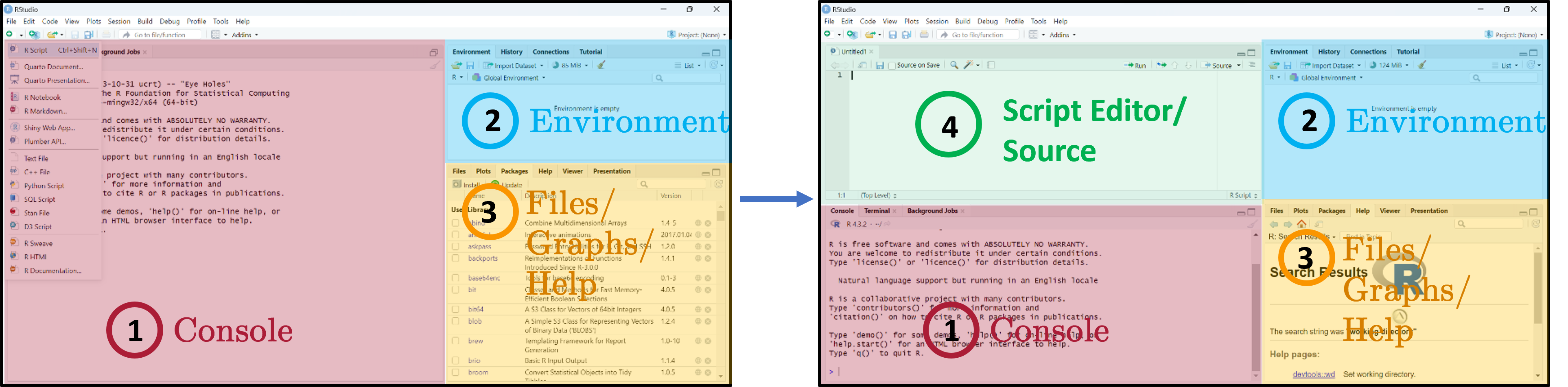
RStudio interface
Three main panes when you open RStudio:
- Console — where R code is executed.
- Global Environment / History — your in-memory objects.
- Files / Plots / Packages / Help / Viewer — the swiss-army-knife pane.
- Script Editor — where you write and save your R scripts.
Writing code in RStudio
- Load and save
.Rscripts. - Keeps a record of your analysis — show others how it was run, repeat later.
- Edit code without accidentally running it.
- Where R code is executed.
- You can also run code interactively here, but it is NOT saved on disk.
- See output and errors directly.
Write and run code through the Script Editor. Use the Console only for quick exploration.
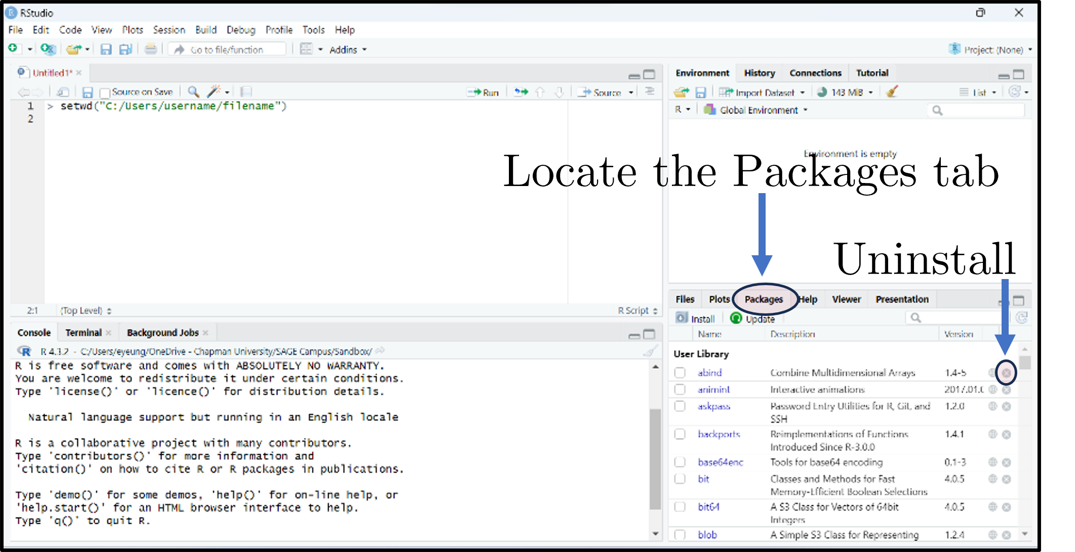
Setting the working directory
- The working directory (
wd) is where R looks for and saves files. - Two ways to set it: via the menu, or in code with
setwd(). - Always verify with
getwd()to avoid confusion about where your files are being read from or written to. - Tip: set the working directory at the start of your script so it’s clear where files are coming from and going to. Avoid hardcoding paths if you plan to share your code with others or run it on different machines.
Getting started — running code
The blinking cursor in the Script Editor prompts you to write. The Console shows > when R is ready.
Four ways to run code:
- Ctrl/Cmd + Enter — run current line / selection.
- Click Run.
- Ctrl + Shift + Enter — run all lines in the editor.
- Highlight lines and click Run.
Short exercise
Type 1 + 2*8 and log(10). Result appears in the Console with a leading [1] (the index of the first element on that line).
What are packages?
- Packages expand what you can do beyond base R.
- A collection of functions, data sets, and other R objects under one name.
- Install from repositories: CRAN, GitHub, etc.
- The Packages tab lists installed packages; click Update to upgrade; the small × uninstalls.
Installing and loading packages
Or click Install in the Packages tab.
Or tick the package’s checkbox in the Packages tab.
Short exercise
Install and load the tidyverse, tidyquant, and Quandl packages.
2.4 Live Coding Session 1
- 2.1 Course objectives
- 2.2 Recap from Lecture 1
- 2.3 Introduction to R
- 2.4 Live Coding Session 1
- 2.M Conclusion of Lecture 2
- Creating objects / variables
- Four data types in R
- Variables and basic operations
- Five basic data structures
- Vectors
- Matrices
- Data frames
- Lists
- Functions
- Loops
- Data import & export — file types
- Data import & export — examples
- Saving your script
- Closing an R session
Creating objects / variables
- The “<-” operator assigns the value on the right to the name on the left.
- Avoid long object names, be descriptive
- Don’t reuse names of existing R functions
- No blank spaces - use
_or. - R is case-sensitive (
xandXare different) - Use
=for function arguments, but “<-” for assignment to avoid confusion - Don’t use
=for assignment in scripts, as it can lead to bugs and readability issues
Four data types in R
- Numeric — numbers that may contain decimals.
- Integer — special case, no decimals (suffix
L).
- Integer — special case, no decimals (suffix
- Character — text (strings); wrap in
" ". - Factor — special character used for categorical data (e.g., male/female, months).
- Logical — Boolean (
TRUE/FALSE).
class(objectname)returns the higher-level label R uses to decide which functions and behaviors apply ("data.frame","factor","matrix","numeric").
Variables and basic operations
- Assign and compute financial metrics — returns, prices, ratios — quickly during empirical work
- Use factors to manage categorical variables like sectors, credit ratings, or time periods
- Logical variables are useful for filtering data frames (e.g.,
subset(myData, myData$sector == "Tech"))
Five basic data structures
- Individual values — single scalars.
- Vectors — ordered collections of elements (one type only).
- Matrices — 2D arrays; rows × columns; one type only.
- Data frames — like spreadsheets; columns can have different types.
- Lists — flexible containers that can hold vectors, matrices, data frames, even other lists.
Vectors
# Create
myVector <- c(3, 4, -1.1, pi)

# Inspect / aggregate
myVector[3]        # third element: -1.1
length(myVector)   # 4
sum(myVector)      # ~9.04
mean(myVector)     # ~2.26
var(myVector)      # ~5.21
sort(myVector)     # ascending: -1.1, 3.0, 3.14, 4.0
quantile(myVector, c(0.1, 0.25, 0.95))

# Vectorized arithmetic — no loops needed
myVector + 2
myVector * myVector

# Coercion: mixed types collapse to character
mixed <- c(1, "two", TRUE)   # "1" "two" "TRUE"

# Named vectors
namedVec <- c(apple = 5, banana = 3)
namedVec["banana"] # 3- Basic syntax:
c()combines values into a vector; indexing with[]retrieves elements - Vectors are the building blocks of more complex structures. They allow you to store and manipulate sequences of numbers, text, or logical values efficiently
- Vectorized operations enable you to perform calculations on entire vectors without writing explicit loops, which is faster and more concise
- Named vectors can improve readability and allow for easier access to specific elements by name rather than index
Matrices
myMatrix <- matrix(c(2, 1, 0, -9, 5, 0), nrow = 2, byrow = TRUE)
dim(myMatrix)              # [1] 2 3
myMatrix[1, 1] <- 2.1415   # modify cell
myMatrix[, 2]              # second column

# Linear algebra
anotherMatrix <- matrix(c(5, -1, 7, 0, 2, -1), nrow = 2, byrow = TRUE)
transposedMatrix <- t(anotherMatrix)
matrixProduct    <- myMatrix %*% transposedMatrix     # 2x2 product
matrixInverse    <- solve(matrixProduct)              # inverse

# Aggregations
rowSums(myMatrix)
colMeans(myMatrix)

# Bind: combine rows / cols
cbind(myMatrix, c(6, 7))- Basic syntax:
matrix()creates a matrix from a vector of values; specifynrowandncolto set dimensions;byrow = TRUEfills by rows instead of columns - Matrices are 2D structures that can only hold one type of data (e.g., all numeric)
- They are essential for linear algebra operations, which are common in finance1
- Functions like
rowSums(),colMeans(), andcbind()allow you to perform common matrix manipulations without writing loops
Data frames
student_name <- c("Student A", "Student B", "Student C")
grade        <- c(1.7, 2.3, 5.0)
students     <- data.frame(student_name, grade)

students$grade                    # column access
colnames(students)[2] <- "exam2021"
students[2:3, ]                   # rows 2-3

# Add columns
students$degree    <- c("Bachelor", "Master", "Bachelor")
students$pass_fail <- c("Pass", "Pass", "Fail")
table(students$degree, students$pass_fail)

# Summary
summary(students)

# Subset by condition
subset(students, exam2021 > 2)

# Add row
newStudent <- data.frame(student_name = "Student D", exam2021 = 3.5,
                         degree = "PhD", pass_fail = "Pass")
students <- rbind(students, newStudent)

# Merge with another frame
ages   <- data.frame(student_name = c("Student A", "Student B", "Student C"),
                     age = c(20, 22, 21))
merged <- merge(students, ages, by = "student_name")- Basic syntax:
data.frame()creates a data frame from vectors; columns can have different types; access with$or[] - Data frames are the most common structure for tabular data in R. They can hold different types of data in different columns (e.g., numeric grades, character names, factors for degree)
- Adding new columns is straightforward, and you can easily summarize or subset the data
- Merging data frames is common when you have related datasets1 that share a key
Lists
scoresList <- list(
  scores = c(95, 85, 92),
  names  = c("Alice", "Bob", "Carol"),
  passed = c(TRUE, TRUE, FALSE)
)

str(scoresList)

scoresList$scores[3] <- 90  # update Carol's score
scoresList$comments  <- "All passed"  # add element

# Nested list
nestedList <- list(course = "Math 101", details = scoresList)
nestedList$details$names[1]  # "Alice"

# Convert to data frame (elements need equal length)
scoresDF <- as.data.frame(scoresList)- Basic syntax:
list()creates a list; access with$or[]; lists can contain any type of object, including other lists - Lists are flexible containers that can hold a variety of objects, making them useful for storing complex data structures or results from functions that return multiple outputs
- They are particularly useful when you want to return multiple related objects from a function without having to combine them into a single data frame or matrix
Functions
# Define
bmiCalc <- function(height, weight) {
  bmi <- weight / (height ^ 2)
  return(round(bmi, 1))
}

# Call
myBmi <- bmiCalc(1.75, 70)   # 22.9

# Default arguments
bmiCalcDefault <- function(height, weight = 70) {
  round(weight / (height ^ 2), 1)
}
bmiCalcDefault(1.75)         # 22.9

# Multiple returns via list
bmiAdvanced <- function(height, weight) {
  bmi <- weight / (height ^ 2)
  category <- ifelse(bmi < 18.5, "Underweight",
                     ifelse(bmi < 25, "Normal", "Overweight"))
  list(bmi = round(bmi, 1), category = category)
}
result <- bmiAdvanced(1.75, 70)
result$bmi        # 22.9
result$category # "Normal"- Basic syntax:
function(arg1, arg2) { ... }defines a function; usereturn()to specify output; functions can have default arguments and return multiple values via lists - Functions allow you to encapsulate reusable code, making your scripts cleaner and more modular
- Functions are essential for performing repeated calculations, especially when you need to apply the same logic to different inputs
Loops
- Basic syntax:
for (var in sequence) { ... }iterates over elements;while (condition) { ... }continues until condition is false - Loops are useful for certain tasks, but in R, they can be inefficient for data manipulation. Whenever possible, use vectorized operations or apply functions instead of loops for better performance
- In practice, you’ll often use functions from packages like
dplyrthat abstract away the need for explicit loops when working with data frames
Data import & export — file types
You will rarely build matrices/data frames by hand. Common ways to read data:
- Text —
.TXT(readLines()) - Tabular —
.CSV,.TSV(read.table(),readr::read_csv()) - Excel —
.XLSX(xlsx,readxl) - Google sheets —
googlesheets4 - Statistics programs — SPSS, SAS (
haven) - Databases — MySQL (
RMySQL)
Data import & export — examples
# CSV
write.csv(objectname, file = "output_file.csv", row.names = FALSE)

# Tab-delimited
write.table(objectname, file = "output_file.txt",
            sep = "\t", row.names = FALSE, col.names = TRUE)

# Excel
library(writexl)
write_xlsx(objectname, "output_file.xlsx")

# RDS
saveRDS(objectname, file = "output_file.rds")
The argument
sep =may not be necessary — R recognises,in.csvand whitespace in.txt. But sometimes R won’t read correctly unless you specify it
Saving your script
- Save every step in an
.Rscript. Comment lines start with#and are ignored at run time. - File → Save, or click the disk icon, or Ctrl/Cmd + S.
- Unsaved scripts (or unsaved edits) show red text and an asterisk in the tab name.
Closing an R session
Three ways to close RStudio:
- File → Quit Session
- The red ✕ in the top-right corner.
- Run
q()in the Console.
Don’t save the workspace image (.RData)
Unless (a) you ran something very expensive, or (b) you’re nearly done with the project. Starting clean each session avoids hidden state from previous runs.
2.M Conclusion of Lecture 2
- 2.1 Course objectives
- 2.2 Recap from Lecture 1
- 2.3 Introduction to R
- 2.4 Live Coding Session 1
- 2.M Conclusion of Lecture 2
- Course at a glance (1/2)
- Course at a glance (2/2)
- Further reading
- Prepare before next lecture
- See you next time
- References
Course at a glance (1/2)
Foundations
Week 1
15.04.2026
Course outline · Backtesting fundamentals
- Course aim & organisation
- Backtesting overview & case study
- In-sample tests (Welch & Goyal 2008)
- Out-of-sample (walk-forward, R²_OS)
- Useful predictors & p-hacking
Introduction to R
Week 2
22.04.2026
RStudio · variables · vectors · data frames · live coding
- Why R for empirical asset-management research
- RStudio and the script editor
- Variables, vectors, matrices, data frames, lists
- Functions and loops
- Data import and export
Assessing model accuracy & Ridge regression
Week 3
29.04.2026
Statistical learning · MSE · bias-variance · linear model selection · Ridge
- Statistical learning: Y = f(X) + ε
- Quality of fit and the train/test MSE distinction
- Bias-variance trade-off and overfitting
- OLS limits: prediction accuracy & interpretability
- Ridge regression and the L2 penalty
Lasso, cross-validation & Elastic Net
Week 4
06.05.2026
Sparse regularisation · resampling for honest test error · choosing λ
- Lasso: L1 penalty and exact-zero coefficients
- Cross-validation: validation set, LOOCV, K-fold
- Choosing the optimal λ for Lasso
- OLS post-Lasso for cleaner coefficient inference
- Elastic Net — combining Ridge and Lasso
Prediction markets, the Polymarket Quant Bench & your project
Week 5
13.05.2026
From Welch-Goyal to event-resolved binary contracts
- Prediction markets — definition and Polymarket as the canonical venue
- How prices form: liquidity, resolution, mechanics
- The Polymarket Quant Bench dataset (HuggingFace): access and schema
- First look at the data in R
- Your project: indicator design, back-test, deliverables, R toolbox
Course at a glance (2/2)
Final presentations
Week 13
01.07.2026
Group presentations · Q&A · wrap-up
- Presentation order and time budget
- Q&A rules
- Closing thoughts and feedback
Further reading
- James et al. (2021) — An Introduction to Statistical Learning with Applications in R (free at https://www.statlearning.com); Chapter 2.3 mirrors today’s R intro.
- Scheuch, Voigt, and Weiss (2023) — Tidy Finance with R — finance-specific tidyverse cookbook, free at https://www.tidy-finance.org/r/.
- Wickham and Çetinkaya-Rundel (2023) — R for Data Science (2nd ed.), free at https://r4ds.hadley.nz.
Prepare before next lecture
- Save today’s live-coding code in a clean
.Rmdfile — practice this format now; the project deliverable is an Rmd. - Read ISLR §2.2 (“Assessing Model Accuracy”) so the vocabulary lands when Andre opens Lecture 3.
- Re-run the demo blocks against a small data set of your own — anything tabular will do (a CSV from Kaggle, a small Quandl pull, etc.).
See you next time
Reminder
- Lecture 3 (29 April 2026): assessing model accuracy, training-vs-test MSE, the bias-variance trade-off, Ridge regression.
- Bring your laptop with R + RStudio installed and the
ISLR,glmnet,splinespackages already loaded.
References

Institute of Strategic Management and Finance · Ulm University